1. deepseek模型学习笔记
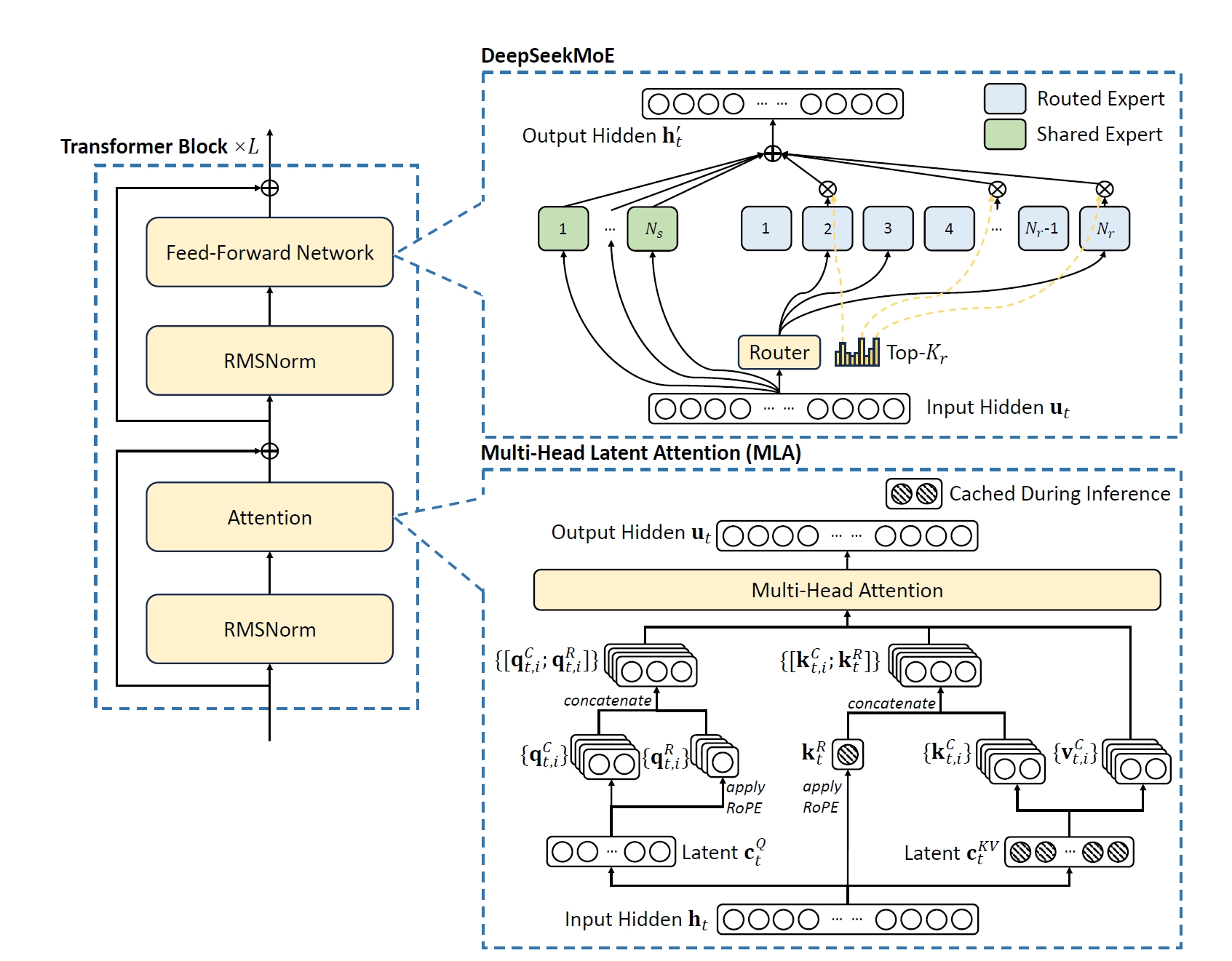
1.1. Multi-Head Latent Attention (MLA)
备注
约定所有计算用行向量,即 \(y = x * W\)
Q的计算公式如下:
where \(\mathbf{c}_{t}^{Q} \in \mathbb{R}^{d_c^{\prime}}\) is the compressed latent vector for queries. \(d_c^{\prime} (\ll d_h n_h)\) denotes the query compression dimension; \(W^{DQ} \in \mathbb{R}^{d \times d_c^{\prime}}, W^{UQ} \in \mathbb{R}^{d_c^{\prime} \times d_h n_h}\) are the down-projection and up-projection matrices for queries, respectively; and \(W^{QR} \in \mathbb{R}^{d_c^{\prime} \times d_h^R n_h}\) is the matrix to produce the decoupled queries that carry RoPE.
KV的计算公式如下:
where \(\mathbf{c}_{t}^{KV} \in \mathbb{R}^{d_c}\) is the compressed latent vector for keys and values; \(d_c (\ll d_h n_h)\) indicates the KV compression dimension; \(W^{DKV} \in \mathbb{R}^{d \times d_c}\) denotes the down-projection matrix; \(W^{UK},W^{UV} \in \mathbb{R}^{d_c \times d_h n_h}\) are the up-projection matrices for keys and values, respectively; \(W^{KR} \in \mathbb{R}^{d \times d_h^R}\) is the matrix used to produce the decoupled key that carries Rotary Positional Embedding (RoPE); \(\operatorname{RoPE}(\cdot)\) denotes the operation that applies RoPE matrices; Note that for MLA, only the blue-boxed vectors (\(\color{blue} \mathbf{c}_{t}^{KV}\) and \(\color{blue}\mathbf{k}_{t}^{R}\)) need to be cached during generation, which results in significantly reduced KV cache while maintaining performance comparable to standard Multi-Head Attention (MHA).
Ultimately, the attention queries (\(\mathbf{q}_{t, i}\)), keys (\(\mathbf{k}_{j, i}\)), and values (\(\mathbf{v}_{j, i}^{C}\)) are combined to yield the final attention output \(\mathbf{u}_{t}\):
where \(W^{O} \in \mathbb{R}^{d_h n_h \times d}\) denotes the output projection matrix.
实际参数大小如下:
d = hidden_size = 7168
\(d_c\) = kv_lora_rank = 512
\(d_c^{\prime}\) = q_lora_rank = 1536
\(n_h\) = num_heads = 128
\(d_h\) = qk_nope_head_dim = 128
\(d_h^R\) = qk_rope_head_dim = 64
\(W^{UQ}\) 和 \(W^{QR}\) 可以合并起来,q_head_dim = qk_nope_head_dim + qk_rope_head_dim = 192. \(W^{DKV}\) 和 \(W^{KR}\) 可以合并起来,kv_lora_rank + qk_rope_head_dim = 576.
1.2. 矩阵吸收absorb
首先考虑如下计算:
其中 \(X\in \mathbb{R}^{m\times d}\) 是输入hidden states, \(A \in \mathbb{R}^{d \times d_c}\) 和 \(B \in \mathbb{R}^{d_c \times n}\) 是权重矩阵, \(C\in \mathbb{R}^{d \times n}\) 是absorb后的等效权重矩阵, 直接计算的flops为:
合并权重后计算的flops为: \(2 m d n\)
当 \(d_c\) 相对较小时,通常导致 \(\boxed{d n \gt d_c (d + n)}\),所以不一定要合并两个权重矩阵!
先不考虑RoPE部分,只考虑从 \(\mathbf{c}^Q\) 和 \(\mathbf{c}^{KV}\) 计算 \(\mathbf{q}_i \mathbf{k}_i^T\) (i表示i-th head)
警告
Absorb 在这的真实含义是矩阵乘法结合律,优先结合 \(\mathbf{q}\) 和 \(W^{UK}\),并缓存 compressed latent vector \(\mathbf{c}^{KV}\), 并不是合并权重矩阵,用 Absorb 命名有一定误导性!
1.2.1. 为什么计算的时候不把 \(W^{UQ}_i (W^{UK}_i)^T\) 合并起来?
可以简单的计算出来对于单个token,单个head所需要的flops分别为: \(2 d_h (d_c^{\prime} + d_c) = 524288\) , \(2 d_c^{\prime} d_c = 1572864 = 3 * 524288\) , 合并后计算量反而是原来的3倍!
1.2.2. 为什么prefill阶段明确计算出k和v,而decode阶段不需要?
假定输入shape如下:
Prefill 阶段 \(s_q = s_{kv} = s\), 可以计算出 Normal 和 Absorb 计算出的flops分别如下:
Decode 阶段 \(s_q = 1, s_{kv} = s\),
从计算量上看,Prefill 阶段 Normal 的计算量比较小,且由于 Prefill 阶段是 计算瓶颈,所以 显式的计算出q和k。
而 Decode 阶段,缓存k cache的时候计算量最小(但会导致kv cache很大), 极限情况是1/4的 Absort 的计算量,但 Decode 瓶颈是 显存带宽。
下面看下两种方式的内存读取量:
Absort 方式的矩阵运算是 \((b, n_h, 1, d_c) \times (b, 1, s, d_c)\),假定为bfloat16精度,读取的memory为
而标准的MHA \((b, n_h, 1, d_h)\times (b, n_h, s, d_h)\) 的内存读取量为:
内存读取比例为:
当 \(s = 20\),访存比值为0.22,极限情况为1/32。所以 Decode 阶段采用了 Absorb 方式计算,并可以复用MQA (Multi-Query Attention) 的实现。
1.2.3. 矩阵吸收问题总结
矩阵吸收的数学问题为 矩阵乘法结合律 该怎么用
其中,A, B, W都是权重。需要权衡计算量,memory读写量和瓶颈,可以套用典型的Roofline Model进行分析。